File:Homotopy with fixed endpoints.png
Jump to navigation
Jump to search
Size of this preview: 525 × 600 pixels. Other resolutions: 210 × 240 pixels | 420 × 480 pixels | 944 × 1,078 pixels.
Original file (944 × 1,078 pixels, file size: 39 KB, MIME type: image/png)
Captions
Captions
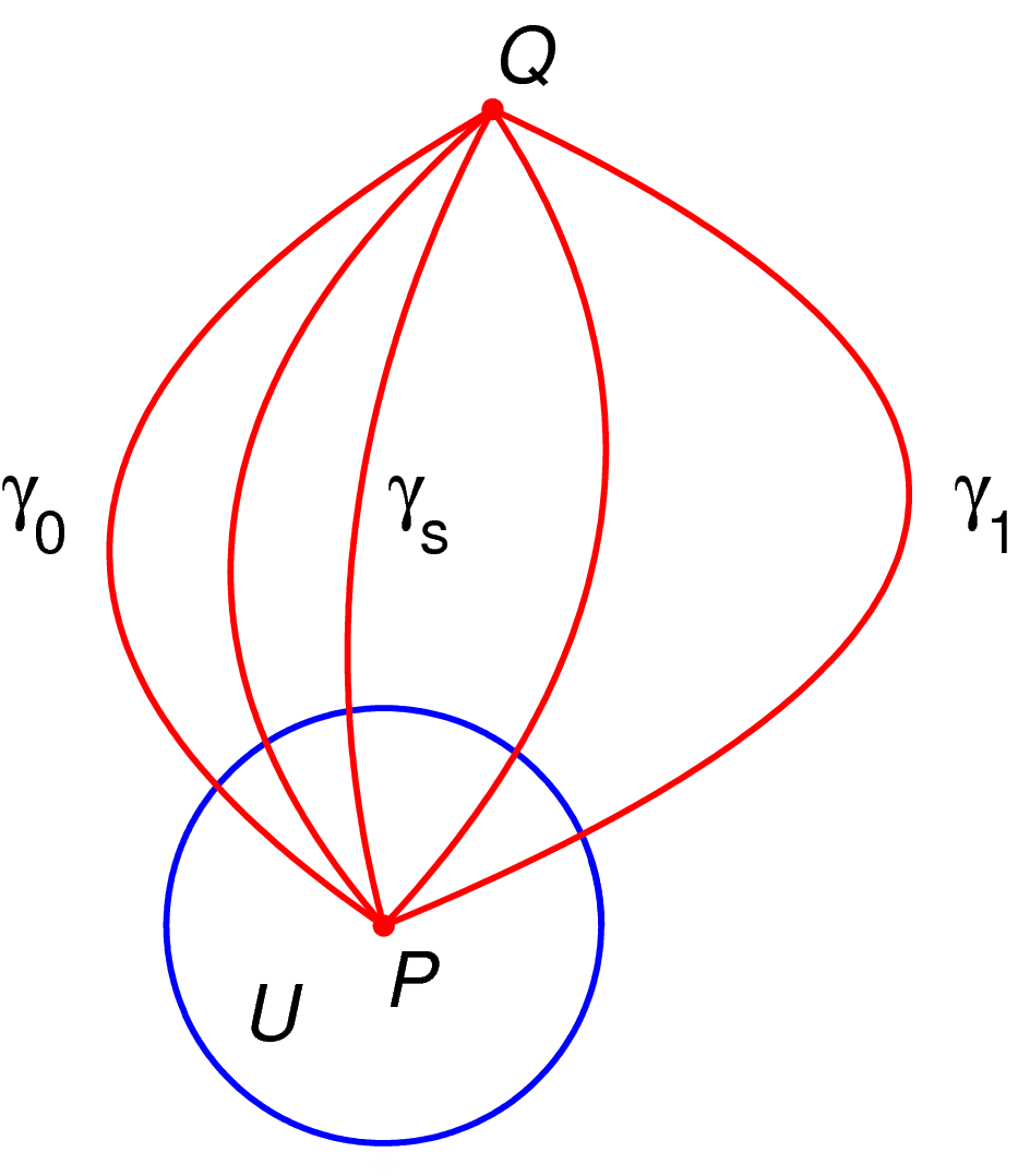
Add a one-line explanation of what this file represents
Made by myself with MATLAB.
| I, the copyright holder of this work, release this work into the public domain. This applies worldwide. In some countries this may not be legally possible; if so: I grant anyone the right to use this work for any purpose, without any conditions, unless such conditions are required by law. |
% illustrate homotopy with fixed endpoints
function main()

   lw=2;  % line width
   fs=25; % font size
   h=1/100;
   tiny = 0.004;
   tinyrad=0.02;
   red = [1, 0, 0];
   white = 0.99*[1 1 1];

   % prepare the figure
   figure(1); clf; hold on; axis equal; axis off;

   % generate the curve on which the analytic continuation will take place
   XX=[-0.1, 0.3, 0.1]; YY=[0, 1, 1.5];
   Y=YY(1):h:YY(length(YY)); X=spline(YY, XX, Y);

   % plot a circle
   rad=0.4; plot_circle(X(1), Y(1), rad, lw)

   % plot the curves
   t=0; X=spline(YY, XX+[0, t, 0], Y); plot(X, Y, 'color', red, 'linewidth', lw);
   t=0.5; X=spline(YY, XX+[0, t, 0], Y); plot(X, Y, 'color', red, 'linewidth', lw);
   t=-0.8; X=spline(YY, XX+[0, t, 0], Y); plot(X, Y, 'color', red, 'linewidth', lw);
   t=-0.6; X=spline(YY, XX+[0, t, 0], Y); plot(X, Y, 'color', red, 'linewidth', lw);
   t=-0.4; X=spline(YY, XX+[0, t, 0], Y); plot(X, Y, 'color', red, 'linewidth', lw);

   % plot text
   N = length(X);
   Nh = floor(N/2);
   text(X(1), Y(1)-tiny*fs, '\it{P}', 'fontsize', fs)
   text(X(N), Y(N)+tiny*fs, '\it{Q}', 'fontsize', fs)
   text(X(Nh)-0.65, Y(Nh), '\gamma_0', 'fontsize', fs)
   text(X(Nh)+0.06, Y(Nh), '\gamma_s', 'fontsize', fs)
   text(X(Nh)+1.1, Y(Nh), '\gamma_1', 'fontsize', fs)
   text(X(1)-0.26, Y(1)-0.16, '\it{U}', 'fontsize', fs)


   % plot some balls for emphasis
   ball(X(1), Y(1), tinyrad, red);
   ball(X(N), Y(N), tinyrad, red);

  % plot a dummy point to avoid having the picture cutt off at edges
  % when saving to eps (a matlab bug)
   plot(X(1), Y(1)-1.1*rad, '*', 'color', white)

   saveas(gcf, 'homotopy_with_fixed_endpoints.eps', 'psc2');

function plot_circle(x, y, r, lw)

   N=100;
   Theta=0:(1/N):2.1*pi;
   X=r*cos(Theta);
   Y=r*sin(Theta);

   plot(x+X, y+Y, 'linewidth', lw);

function plot_text(x, y, shiftx, shifty, str, fs, tinyrad, color)
   text(x+shiftx, y+shifty, str, 'fontsize', fs);
   ball(x, y, tinyrad, color);

function ball(x, y, r, color)
   Theta=0:0.1:2*pi;
   X=r*cos(Theta)+x;
   Y=r*sin(Theta)+y;
   H=fill(X, Y, color);
   set(H, 'EdgeColor', 'none');

|
This math image could be re-created using vector graphics as an SVG file. This has several advantages; see Commons:Media for cleanup for more information. If an SVG form of this image is available, please upload it and afterwards replace this template with
{{vector version available|new image name}}.
It is recommended to name the SVG file “Homotopy with fixed endpoints.svg”—then the template Vector version available (or Vva) does not need the new image name parameter. |
File history
Click on a date/time to view the file as it appeared at that time.
| Date/Time | Thumbnail | Dimensions | User | Comment | |
|---|---|---|---|---|---|
| current | 01:45, 9 April 2007 | | 944 × 1,078 (39 KB) | Oleg Alexandrov (talk | contribs) | Made by myself with MATLAB. {{PD-self}} |
| 01:39, 9 April 2007 |  | 925 × 1,053 (39 KB) | Oleg Alexandrov (talk | contribs) | Made by myself with MATLAB. {{PD-self}} | |
| 01:39, 9 April 2007 |  | 925 × 1,053 (39 KB) | Oleg Alexandrov (talk | contribs) | Made by myself with MATLAB. {{PD}} |
You cannot overwrite this file.
File usage on Commons
There are no pages that use this file.
File usage on other wikis
The following other wikis use this file:
- Usage on en.wikipedia.org