File:Mean estimator consistency.gif
Mean_estimator_consistency.gif (800 × 325 pixels, file size: 4.53 MB, MIME type: image/gif, looped, 250 frames, 25 s)
Captions
Captions
Summary
[edit]| DescriptionMean estimator consistency.gif |
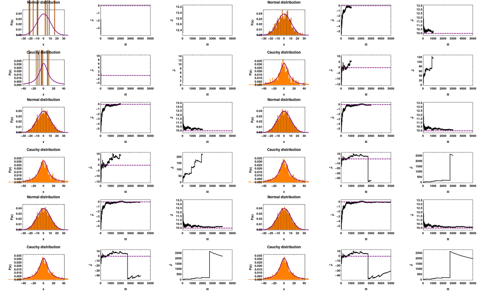
English: If you sample from a Cauchy distribution, the probability to get a value very far on the tails is so high that more data won't ever give you a better estimate of its mean. |
| Date | |
| Source | https://twitter.com/j_bertolotti/status/1303999888137613312 |
| Author | Jacopo Bertolotti |
| Permission (Reusing this file) |
https://twitter.com/j_bertolotti/status/1030470604418428929 |
Mathematica 12.1 code
[edit]n = 5 10^3;
data = RandomVariate[NormalDistribution[0, 10], n];
data2 = RandomVariate[CauchyDistribution[0, 10], n];
p0 = Table[
GraphicsGrid[{
{Show[
Histogram[data[[1 ;; j]], {1}, "Probability", ChartStyle -> Orange],
Plot[PDF[NormalDistribution[0, 10], x], {x, -40, 40}, PlotRange -> All, PlotStyle -> {Purple, Thick}]
, PlotRange -> {{-30, 30}, {0, 0.045}}, Axes -> False, Frame -> True, FrameLabel -> {"x", "P(x)"}, LabelStyle -> {Black, Bold}, PlotLabel -> "Normal distribution"
]
,
ListPlot[Table[Mean[data[[1 ;; i]] ], {i, 9, j}], Joined -> True, PlotRange -> {{0, n}, All}, DataRange -> j, Axes -> False, Frame -> True, FrameLabel -> {"#", "\!\(\*OverscriptBox[\(\[Mu]\), \(^\)]\)"}, LabelStyle -> {Black, Bold}, PlotStyle -> Black, Epilog -> {Purple, Thick, Dashed, Line[{{0, 0}, {n, 0}}]}]
,
ListPlot[Table[StandardDeviation[data[[1 ;; i]] ], {i, 9, j}], Joined -> True, PlotRange -> {{0, n}, All}, DataRange -> j, Axes -> False, Frame -> True, FrameLabel -> {"#", "\!\(\*OverscriptBox[\(\[Sigma]\), \(^\)]\)"}, LabelStyle -> {Black, Bold}, PlotStyle -> Black, Epilog -> {Purple, Thick, Dashed, Line[{{0, 10}, {n, 10}}]}]
}, {
Show[
Histogram[data2[[1 ;; j]], {1}, "Probability", ChartStyle -> Orange],
Plot[PDF[CauchyDistribution[0, 10], x], {x, -40, 40}, PlotRange -> All, PlotStyle -> {Purple, Thick}], PlotRange -> {{-40, 40}, {0, 0.035}}, Axes -> False, Frame -> True, FrameLabel -> {"x", "P(x)"}, LabelStyle -> {Black, Bold}, PlotLabel -> "Cauchy distribution"]
,
ListPlot[Table[Mean[data2[[1 ;; i]] ], {i, 1, j}], Joined -> True, PlotRange -> {{0, n}, All}, DataRange -> j, Axes -> False, Frame -> True, FrameLabel -> {"#", "\!\(\*OverscriptBox[\(\[Mu]\), \(^\)]\)"}, LabelStyle -> {Black, Bold}, PlotStyle -> Black, Epilog -> {Purple, Thick, Dashed, Line[{{0, 0}, {n, 0}}]}]
,
ListPlot[Table[StandardDeviation[data2[[1 ;; i]] ], {i, 2, j}], Joined -> True, PlotRange -> {{0, n}, All}, DataRange -> j, Axes -> False, Frame -> True, FrameLabel -> {"#", "\!\(\*OverscriptBox[\(\[Sigma]\), \(^\)]\)"}, LabelStyle -> {Black, Bold}, PlotStyle -> Black]
}}, ImageSize -> 800]
, {j, 10, n, 20}];
ListAnimate[p0]
Licensing
[edit]| This file is made available under the Creative Commons CC0 1.0 Universal Public Domain Dedication. | |
| The person who associated a work with this deed has dedicated the work to the public domain by waiving all of their rights to the work worldwide under copyright law, including all related and neighboring rights, to the extent allowed by law. You can copy, modify, distribute and perform the work, even for commercial purposes, all without asking permission.
http://creativecommons.org/publicdomain/zero/1.0/deed.enCC0Creative Commons Zero, Public Domain Dedicationfalsefalse |
File history
Click on a date/time to view the file as it appeared at that time.
| Date/Time | Thumbnail | Dimensions | User | Comment | |
|---|---|---|---|---|---|
| current | 09:26, 11 September 2020 | 800 × 325 (4.53 MB) | Berto (talk | contribs) | Uploaded own work with UploadWizard |
You cannot overwrite this file.
File usage on Commons
The following page uses this file:
File usage on other wikis
The following other wikis use this file:
- Usage on en.wikipedia.org
- Usage on simple.wikipedia.org
- Usage on sq.wikipedia.org
Metadata
This file contains additional information such as Exif metadata which may have been added by the digital camera, scanner, or software program used to create or digitize it. If the file has been modified from its original state, some details such as the timestamp may not fully reflect those of the original file. The timestamp is only as accurate as the clock in the camera, and it may be completely wrong.
| GIF file comment | Created with the Wolfram Language : www.wolfram.com |
|---|
